Okay, here’s the deal.

I love trail running, and spend a lot of time in the woods at my local parks, running anywhere from just a few to 20+ miles depending on training. A lot of park maps, however, make it nearly impossible to determine an appropriate route before setting out. Consider for example, this fantastic park near Madison, WI. (One note- this problem has been in the back of my mind for a few years now, and in the time since, they’ve updated their map to solve the issue laid out here, but this older map still suffices to illustrate the point).

Unhelpful Distances

Trying to piece together a 20 mile run is made very difficult by not having point-to-point mileage. While you can ballpark it, trail mileage tends to vary widely with terrain and a smooth dashed line on a map may not represent the actual mileage very closely.

I should be able to do a better job! With a running watch, every trip to a park gives me data on its trails. If I can stitch these together, I should be able to generate my own park map. By detecting junctions, I can break a park up into trail segments and generate a map with individual segments’ mileage marked. Getting the GPS data is the easy (and fun) part. Figuring out how to smooth the data and identify junctions turns out to be much more difficult (but still fun). This problem also illustrates an interesting case where something conceptually simple turns out to be very difficult to implement in a code. Edge cases abound, and I’m constantly faced with the fact that while I’m struggling to develop a reliable method, a human posed with the same problem could do it easily.

Working with the data

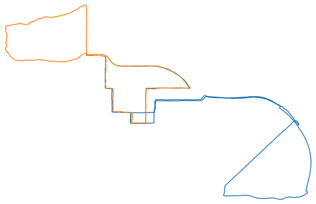
To develop the code to handle processing park runs into a single map, I am working with these two runs.

Two runs to use for code development

Visually this task is simple. I could very easily identify junctions and the segments between them. But dealing with the actual arrays of GPS data, how do you know where the junctions are? When I said before that edge cases abound, it’s more accurate to describe this as an apparently simple task at first and then nothing but edge cases upon closer inspection. But I’ve made significant progress. Here’s my method.

class Park:

    def __init__(self, park_direc, name='blank'):
        self.name = name
        self.junctions = []
        self.segments = []
        self.analyze_park_runs(park_direc)

    def analyze_park_runs(self, park_direc):
        park_runs = extract_park_runs_coords(park_direc)
        for run in park_runs:
            self.analyze_run(park_runs[run], run)

    def analyze_run(self, coords, runname):

        # step 1- segment on known junctions
        broken_up_segs = self.segment_on_junctions(coords)

        # step 2- compare resulting segments with known segments, average into if same
        for seg in broken_up_segs:
            sameas = self.compare_to_known_segments(seg)
            if sameas is None:  # new segment
                newjuncs, weights = self_compare(seg)  # check for new juncs in new segment
                if len(newjuncs) == 0:  # no new juncs, add as new segment
                    self.add_new_segment(seg, runname)
                else:
                    for (nj, wt) in zip(newjuncs, weights):
                        self.junctions.append(Junction(nj[1], nj[0], wt, runname))
                    self.analyze_run(coords, runname)  # send through again with new junctions known
            else:
                self.fold_into(sameas, seg)

We’re creating a class object for each park, which will eventually hold arrays of junctions and segments. Each junction and segment is also a class object, with relevant data including GPS data, weight, and the run in which it was first identified. In the initialization of the Park object we call analyze_park_runs which will iterate through all the GPS files in the given directory and analyze them separately. The analysis of each run is done in two steps. First, we segment the run on known junctions. If this is the first run analyzed this returns the run in its entirety, having no junctions on which to break it up, but otherwise returns an array of segments. In step 2 we iterate through the segments and begin by comparing them to known segments. All segments and junctions have a unique ID, and as each segment has start/end junctions identified, we begin by comparing the start/end junctions of the segments we’re comparing. If the two junctions are the same, we do a distance comparison to check whether the two segments diverge significantly. (This word significantly factors heavily into this entire analysis. There are multiple distance variables that are set that determine what “close enough” or “disjoint” might mean, and these sensitivity controls need to be tweaked in order for the code to function as desired). After iterating through the known segments there are two possible outcomes. If a segment was found with the same endpoints and no significant deviation between the two, they’re considered the same and the new segment is folded into the existing one. If no segment was found to match the one under consideration then this new segment is analyzed further. So far this has been a pretty straightforward problem. This part of the analysis, however, highlights the two biggest challenges of this coding problem.

Challenge the first: how to identify junctions

This first big challenge is how to locate junctions in the data. Again, this is a very easy task to accomplish visually, but coding it up is a real difficulty. We want to smooth out the data to allow some tolerance, since two portions of the route that are obviously the “same” will never have exactly the same GPS coordinates, so we need some sense of “closeness” in the analysis. But we need to identify where two portions of the route diverge, so we need some sense of how much is enough to consider them distinct? Below is my method. It takes in a segment and, comparing only to itself, looks for new junctions. (Of note at this time I don’t have a method to identify junctions between two different segments, but this will be implemented soon).

def self_compare(seg: BrokenSegment):  # compares a segment with itself to look for junctions
    lon, lat = seg.lon_arr, seg.lat_arr
    avlat = np.mean(lat)
    dlon = rsearch / (rearth * np.cos(avlat * dtor)) / dtor  # [deg]
    # dist.distance takes [lat, lon] as input
    delta = np.array([dist.distance([lat[i], lon[i]], [lat[i + 1], lon[i + 1]]).m for i in np.arange(len(lon) - 1)])
    nsmooth = np.ceil(np.log2(max(delta)))  # subdivide so steps are < 1 m
    lon, lat, delta = clean_subdivide(lon, lat, delta, nsmooth)  # just adds in midpoints, no smoothing
    delta = np.append(0., delta)  # throw 0 out front so delta lines up with lat/lon array
    cumdist = np.nancumsum(delta)  # cumulative route distance

    loop = dist.distance([lat[0], lon[0]], [lat[-1], lon[-1]]).m < rsearch

    juncs = []
    scanning = True
    ipos = 0
    while scanning:
        ptstat, _ = determine_pt_status(lon, lat, dlon, dlat, ipos, cumdist, loop, verbose=True)
        posptstat = ptstat

        # big moves
        ijump = 500  # jump some pts and check again
        while posptstat == ptstat:
            ipos += ijump
            if ipos >= len(lon):
                scanning = False
                break
            posptstat, _ = determine_pt_status(lon, lat, dlon, dlat, ipos, cumdist, loop)

        # small moves
        posptstat, ipos = ptstat, ipos - ijump  # reset and check again
        ijump = 1  # jump some pts and check again
        while posptstat == ptstat:
            ipos += ijump
            if ipos >= len(lon):
                scanning = False
                break
            posptstat, _ = determine_pt_status(lon, lat, dlon, dlat, ipos, cumdist, loop)

        if ipos < len(lon):
            juncs.append([lon[ipos], lat[ipos]])  # [lon, lat]
        print('looping')

    juncs_merged, weights = [], []
    ijunc2scan = np.arange(len(juncs))
    while len(ijunc2scan) > 0:
        jdist = [dist.distance(juncs[ijunc2scan[0]][::-1], juncs[iij][::-1]).m for iij in ijunc2scan]
        iav = np.where(np.array(jdist) < junc_merge_dist)  # merge juncs within junc_merge_dist
        avgd_junc = np.mean(np.array(juncs)[ijunc2scan[iav]], axis=0)
        juncs_merged.append(avgd_junc)
        weights.append(len(iav[0]))
        ijunc2scan = np.setdiff1d(ijunc2scan, ijunc2scan[iav])
    return juncs_merged, weights

I begin by adding a bunch of midpoints to each segment to ensure that the steps are less than 1 m (clean_subdivide). The routine then scans through the entire array. The determine_pt_status method identifies whether or not there is another portion of the run nearby. In the orange run in the image above, you can see there are basically two lobes with an overlapped stretch in the middle. So while on either of those two lobes, determine_pt_status returns alone and in the overlapped portion returns there is another (it actually returns 1 or 2 but the descriptive is more fun). It continues scanning, first using larger jumps to reduce the number of comparisons that need to be made, until the status changes. When it changes it then goes back a step and scans forward one point at a time to identify the exact index at which the point status changes, then adds this as the location of a junction. As a last step it then goes through and averages together junctions that are near each other. This is because, in the run in orange above, we go through each junction twice, once on the way out and once on the way in, and we take the GPS locations we identified using the pt_status and average together the outbound and inbound locations to give us a better estimate for the actual junction location.

Challenge the second: how to intelligently average GPS data

The second challenge is when we identify two segments that are the same, how do we average them together? This feels like it’d be obvious, but the data is irregular, and again we have to be careful about some edge cases. We can’t average together based on time since my pace varies, and averaging together based on some longitude/latitude window is not a bad idea but would pull the endpoints of the segments away from the junctions. Instead I use the distance from one of the junctions as my comparator (this has its issues, see known issues below). These are, after all, supposed to be the same segment of trail, so I start at Junction1 and go to Junction2. How long I take to get there, even if I go back and forth a few times (“did I lock my car?”) or any other unforeseen data weirdness, my longitude and latitude should be tied to my distance from one of the endpoints. So in the code below, I compute this distance array for each of the segments (I’ve already checked to ensure they’re directionally aligned), then create corresponding x arrays on the interval [0,1] (here actual distance doesn’t matter since both segments traverse the same distance between their start/endpoints. I create the interpolation axis xint based on the previously computed distance of the known segment so that we are well-sampled, then simply interpolate the lat/lon arrays onto this new axis. This is a simple linear interpolation. GPS data can be quite erratic and I have avoided any smoothing of the data at this point. A simple averaging of the two segments now gives a good result.

def fold_together(lon1, lat1, lon2, lat2, known_dist):
    d1 = [dist.distance([lat1[0], lon1[0]], [lat1[i], lon1[i]]).m for i in np.arange(len(lon1))]
    d2 = [dist.distance([lat2[0], lon2[0]], [lat2[i], lon2[i]]).m for i in np.arange(len(lon2))]
    x1, x2 = np.linspace(0, 1, num=len(d1)), np.linspace(0, 1, num=len(d2))

    xint = np.linspace(0, 1, num=int(known_dist * 2))  # set for roughly 1/2 m interval
    ilon1, ilat1 = np.interp(xint, x1, lon1), np.interp(xint, x1, lat1)
    ilon2, ilat2 = np.interp(xint, x2, lon2), np.interp(xint, x2, lat2)
    ilon, ilat = (ilon1 + ilon2) / 2., (ilat1 + ilat2) / 2.

    return ilon, ilat

Progress

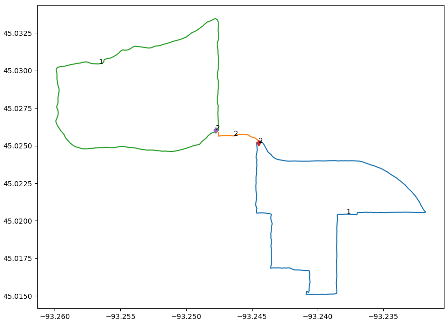
Utilizing the methods outlined above, I’ve so far run this analysis on just the orange run from the image above. The result is shown below. Processing of single run

Each segment is shown in a different color, with the weight annotated near the middle, and each junction likewise has its weight shown. As desired, the code has identified 3 different segments and 2 junctions. Each junction has weight 2 (from averaging the outbound/inbound portion) and the overlapped segment also has weight 2. Some obvious notes on the status of the code: The segments do not include their endpoints when plotted, so we see gaps in the data. The segments do not exactly look like they’re going to pass through their junctions, but this should improve as more data is added. After all, the lower right and upper left segment are based on only one data source and so have not been averaged together at all.
It’s not all that impressive to look at, but this represents significant progress! I’m very happy with it :)

Known Issues

This is still very much a work in progress. A few things are known to remain that need to be addressed. (Many more probably exist that are not known).

• The averaging method used works well on segments where the distance from an endpoint is monotonic towards the other. For the two lobes shown above, the distance arrays would be double-valued, and the lat/lon of the return portion would be averaged together with the outbound portion.
• I currenly do not have a method for identifying new junctions between two segments, they are only identified during the self_compare method.